Machine-Learning-Lab1

实验介绍

在本练习中，您将实现线性回归，并了解它的工作原理

实验文件：

• ex1.m - Octave/MATLAB脚本，帮助您完成练习
• ex1 multi.m - 多个 Octave/MATLAB 脚本，用于练习的后续部分
• ex1data1.txt - txt-单变量线性回归数据集
• ex1data2.txt - txt-多变量线性回归数据集
• submit.m - 将您的解决方案发送到我们的服务器
• [?] warmUpExercise.m - Octave/MATLAB中的简单示例函数
• [?] plotData.m - 用来显示数据集的函数
• [?] computeCost.m - 用来计算线性回归的成本的函数
• [?] gradientDescent.m - 用来运行梯度下降的函数
• [†] computeCostMulti.m - 多变量代价函数
• [†] gradientDescentMulti.m - 多变量梯度下降
• [†] featureNormalize.m - 用于规范化特征的函数
• [†] normalEqn.m - 用于计算正规方程组的函数

在整个练习中，您将使用 ex1.m 和 ex1 multi.m，这些脚本为问题设置数据集，并调用将要编写的函数，您不需要修改它们中的任何一个，您只需按照本任务中的说明修改其他文件中的函数

对于这个编程练习，您只需要完成练习的第一部分，就可以使用一个变量实现线性回归，练习的第二部分是可选的，内容包括使用多变量

PS：由于本人不会使用 Octave，以下实验是在 github 上找的 python 版本

Linear regression with one variable（单变量线性回归）

在本练习的这一部分中，您将使用一个变量实现线性回归，以预测食品卡车的利润：

• 假设你是一家连锁餐厅的首席执行官，正在考虑在不同的城市开设一家新的分店
• 这家连锁店在各个城市都有卡车，你可以从这些城市获得利润和人口数据
• 您希望使用这些数据来帮助您选择下一步要扩展到哪个城市
  • 文件 ex1data1.txt 包含线性回归问题的数据集（第一列是一个城市的人口，第二列是该城市食品卡车的利润，利润为负值表示亏损）
  • 脚本 ex1.m 已经被设置好你需要加载的这些数据

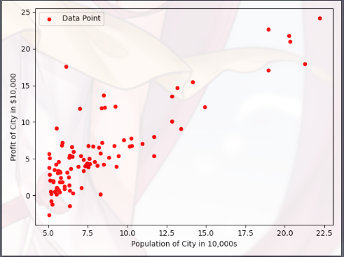
Plotting the Data A（绘制数据）

在开始任何任务之前，通过可视化来理解数据通常是有用的

对于这个数据集，您可以使用散点图来可视化数据，因为它只有两个属性需要绘制 - 利润和人口（你在现实生活中会遇到的许多其他问题都是多维的，无法绘制在二维图上）

• 在 ex1.m 中，数据集从数据文件加载到了变量X和Y中：

import matplotlib.pyplot as plt # as相当于加了一个别称(这个类不用实例化)

# ======== 1.载入数据和绘制散点图 ========
print('读取数据，并绘制散点图...\n')
filepath = r'data\ex1data1.txt'
# 从文件中读取数据,第一列是城市的人口,第二列是该城市食品卡车的利润,中间用','作为分隔符
dataset = np.loadtxt(filepath, delimiter=',', usecols=(0,1)) 
# filepath: 文件路径
# delimiter: 分隔符
# usecols: 选取数据的列编号
Xdata = dataset[:,0] # 获取第一列的数据-城市的人口(因)
Ydata = dataset[:,1] # 获取第二列的数据-卡车的利润(果)
plt.figure(0) # 初始化图表(命名其为"0")
plt.scatter(Xdata,Ydata,c='red',marker='o',s=20) # 设置图表上的断点
plt.xlabel('Population of City in 10,000s',fontsize=10) # 设置x轴上的文字
plt.ylabel('Profit of City in $10,000',fontsize=10) # 设置y轴上的文字
plt.legend(['Data Point']) # 设置左上角的注释
plt.show() # 显示该图表

• loadtxt(filepath , delimiter , usecols)：从文件路径 filepath 中读取第 usecols 列的数据，以 delimiter 为数据之间的间隔

这里使用了 Matplotlib Pyplot 模块（Pyplot 是常用的绘图模块，能很方便让用户绘制 2D 图表）

Gradient Descent（梯度下降）

• 算法原理：

$$repeat\,\,\, until\,\,\, convergence\{ \\ θ_j:=θ_j-\alpha\frac∂{∂θ_j}J(θ_0,θ_1)\quad(for\,\,\,j=0\,\,\,and\,\,\,j=1) \\ \}$$

• 代码实现：

import numpy as np
from computeCost import compute_cost

def gradient_descent(X,Y,theta_init,alpha,iter_num):
    # X: 城市的人口(添加有偏置维度)
    # Y: 卡车的利润
    # theta_init: 参数θ(初始值)
    # alpha: 学习率α
    # iter_num: 迭代次数iter
    m = Y.shape[0] 
    J_history = np.zeros(iter_num) # 用于记录代价的历史值
    theta = theta_init
    for num in range(0,iter_num): 
        J_history[num] = compute_cost(X,Y,theta) # 用代价函数计算代价并记录
        hyp = np.dot(X,np.transpose(theta))
        theta = theta - alpha * np.dot(np.transpose(hyp -Y),X) / m 
    return theta,J_history # 返回"参数θ(已改变)"和"代价的历史值"

• zeros()：返回来一个给定形状和类型的，用“0”填充的数组
• shape()：它的功能是读取矩阵的长度，比如 “shape[0]” 就是读取矩阵第一维度的长度

Mean squared error（代价函数-均方误差）

• 算法原理：

$$J(θ_0,θ_1)= \frac1{2m}\sum_{i=1}^m(\hat y^{(i)}−y^{(i)})^2= \frac1{2m}\sum_{i=1}^m(h_θ(x^{(i)})−y^{(i)})^2$$

• 代码实现：

import numpy as np

def compute_cost(X,Y,theta):
    # X: 城市的人口(添加有偏置维度)
    # Y: 卡车的利润
    # theta: 参数θ(已改变)
	hypthesis = np.dot(X,np.transpose(theta))
	cost = np.dot(np.transpose(hypthesis - Y),(hypthesis -Y))
	cost = cost / (2 * X.shape[0])
	return cost

• dot(x , y)：两个数组作矩阵乘积，当两个数组的维度不能直接进行矩阵乘法时，dot会把尝试后面的参数进行转置
• transpose(x)：把矩阵进行转置

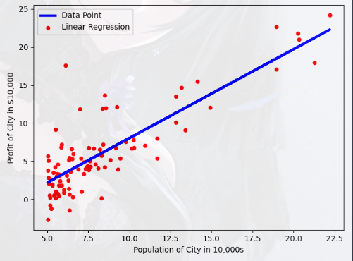
Completion process（具体的拟合过程）

import numpy as np

# ======== 2.计算代价和梯度 ========
print('进行梯度计算...\n')
X = np.c_[np.ones(Xdata.shape[0]),Xdata] # 给输入数据Xdata增加一个偏置维度
Y = Ydata
theta_init = np.zeros(X.shape[1]) # 初始化(θ,参数)
iter_num = 1500 # 初始化(iter,迭代次数)
alpha = 0.01 # 初始化(α,学习率)

print('Initial cost:', str(compute_cost(X,Y,theta_init)), '\nThis value should be 32.07') # 利用代价函数计算初始代价
theta_fin,J_history = gradient_descent(X,Y,theta_init,alpha,iter_num) # 利用梯度下降法进行优化求解,返回记录代价历史值的J_history,和最终θ(theta_fin)
print('Theta found by gradient descent:',str(theta_fin.reshape(2)))

# 绘制数据散点图和线性回归曲线
plt.figure(1)
plt.scatter(Xdata,Ydata,c='red',marker='o',s=20)
plt.plot(X[:,1],np.dot(X,theta_fin),'b-',lw=3)
plt.xlabel('Population of City in 10,000s',fontsize=10)
plt.ylabel('Profit of City in $10,000',fontsize=10)
plt.legend(['Data Point','Linear Regression'])
plt.show()

• ones(shape , dtype=None , order=’C’)：返回给定形状和数据类型的新数组

• c_[ x , y ]：按列叠加两个矩阵，把两个矩阵左右组合，要求行数相等

x_1 = 
 [[1 2 3]
  [4 5 6]]
x_2 = 
 [[3 2 1]
  [8 9 6]]
x_new = 
 [[1 2 3 3 2 1]
  [4 5 6 8 9 6]]

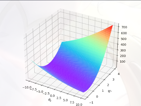
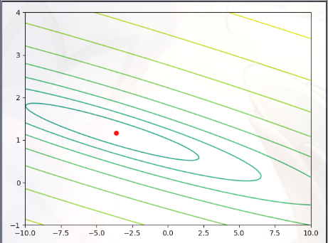
Visualizing J(θ)（可视化代价函数的执行过程）

为了更好地理解代价函数 J（θ），我们将生成 J（θ）的曲面和等高线图

from mpl_toolkits.mplot3d import Axes3D
from matplotlib.colors import LogNorm

# ======== 3.可视化代价J(theta0,theta1) ========
theta0_vals = np.linspace(-10,10,100) # xs的每一行都是theta0_vals的复制
theta1_vals = np.linspace(-1,4,100) # ys的每一列都是theta1_vals的复制
xs,ys = np.meshgrid(theta0_vals,theta1_vals) # 生成网格点坐标矩阵
J_vals = np.zeros(xs.shape)

for i in range(0,theta0_vals.size):
	for j in range(0,theta1_vals.size):
		t = np.array([theta0_vals[i],theta1_vals[j]])
		J_vals[i][j] = compute_cost(X,Y,t)
J_vals = np.transpose(J_vals)

# 绘制3D曲面图
figure = plt.figure(2)
ax = Axes3D(figure) # 把图像指定为3D视图
ax.plot_surface(xs,ys,J_vals,cmap='rainbow') # 指定图形的色彩(彩虹色)
plt.xlabel(r'$\theta_0$')
plt.ylabel(r'$\theta_1$')
plt.show()

# 绘制代价的等高椭圆线
plt.figure(3)
lvls = np.logspace(-2, 3, 20)
plt.contour(xs, ys, J_vals, levels=lvls, norm = LogNorm()) # 设置坐标和值,指定等高线的值,指定色彩
plt.plot(theta_fin[0], theta_fin[1], 'ro',markersize =6) # 设置图像中的那个红点
plt.show()

• linspace(start , stop , num=50 , endpoint=True , retstep=False , dtype=None)：用于在线性空间中以均匀步长生成数字序列
• meshgrid(theta0_vals , theta0_vals)：生成坐标矩阵
• array(A , B , …. )：创建一个数组（参数有几个就是几维）
• logspace(start , stop , num=50 , endpoint=True , base=10.0)：把范围是 “[base的start次方,base的stop次方]” 的数据，在对数尺度上返回间隔均匀的数字（有点看不懂）

>>> np.logspace(2.0, 3.0, num=4)
array([ 100.        ,  215.443469  ,  464.15888336, 1000.        ])
>>> np.logspace(2.0, 3.0, num=4, endpoint=False) # endpoint:停止时是否是最后一个样本
array([100.        ,  177.827941  ,  316.22776602,  562.34132519])
>>> np.logspace(2.0, 3.0, num=4, base=2.0)
array([4.        ,  5.0396842 ,  6.34960421,  8.        ])

结果如下：

Linear regression with multiple variables（多元线性回归）

在这一部分中，您将使用多变量线性回归来预测房价：

• 假设你要卖房子，你想知道一个好的市场价格是多少
• 一种方法是首先收集最近售出房屋的信息，并制作一个房价模型
  • 文件 ex1data2.txt 包含 Portland 房价的培训数据集（第一栏是房子的大小，第二栏是卧室的数量，第三栏是房子的价格）
  • 脚本 ex1_multi.m 已设置脚本以帮助您逐步完成此练习

Feature Normalization（特征规范化）

脚本 ex1_multi.m 首先加载并显示此数据集中的一些值，通过查看这些值，注意到：房屋大小大约是卧室数量的1000倍

当特征相差几个数量级时，首先执行特征缩放可以使梯度下降更快地收敛

Feature Normalization 的原理

• 从数据集中减去每个特征的平均值
• 减去平均值后，再将特征值按各自的“标准偏差”进行缩放（除）

Feature Normalization 代码实现：

def feature_normalize(Xdata):
	X_mean = np.mean(Xdata,axis=0)
	X_std = np.std(Xdata,axis=0)
	X_norm = np.divide(np.subtract(Xdata,X_mean),X_std)

	return X_norm,X_mean,X_std

• mean(A , axis=0)：计算每一维度的均值
• std(A , axis=0)：计算沿指定轴的标准差
• divide(A , B)：数组对应位置元素进行除法
• subtract(A , B)：数组对应位置元素进行减法

Completion process（具体过程）

# ======== 1.读取数据并标准化数据的特征 ========
data = np.loadtxt(r'data\ex1data2.txt',delimiter =',') # 从文件中读取数据,中间用','作为分隔符(第一栏是房子的大小，第二栏是卧室的数量，第三栏是房子的价格)
Xdata = data[:,0:2] # 房子的大小&卧室的数量(因)
Ydata = data[:,2] # 房子的价格(果)
X,mu,sigma = feature_normalize(Xdata) # 对输入数据特征进行标准化
print('Mu is:',mu)
print('Sigma is:',sigma)
X = np.c_[np.ones(X.shape[0]),X] # 给输入数据Xdata增加一个偏置维度
Y = Ydata

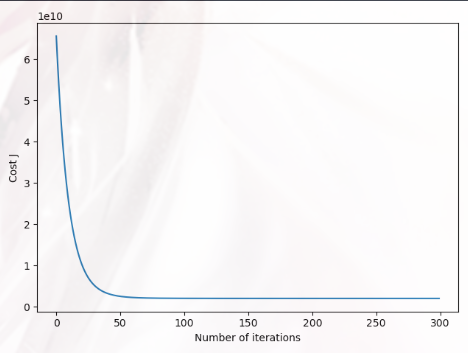
Plotting the Data B（绘制数据）

这一部分我们需要绘制反应 “迭代次数和代价函数值关系” 的图形，还是使用梯度下降法求解：

from gradientDescent import gradient_descent as gd

# ======== 2.使用梯度下降法求解 ========
theta_init = np.zeros(X.shape[1])
alpha = 0.05
num_iters = 300

theta,J_history = gd(X,Y,theta_init,alpha,num_iters) # 利用梯度下降法进行优化求解,返回记录代价历史值的J_history,和最终θ(theta)

# 绘制"迭代次数和代价函数值关系"的图形
plt.figure()
plt.plot(np.arange(J_history.size),J_history)
plt.xlabel('Number of iterations')
plt.ylabel('Cost J')
plt.show()
print('Theta computed from gradient descent : \n{}'.format(theta)) # PS:theta是数组格式

梯度下降算法和前面实现的一样，就不多赘述了，下面是“预测”的过程：

# ======== 3.预测 ========
Xtest = np.array([1,1650,3])
price = np.dot(Xtest,np.transpose(theta))
print('Predicted price of a 1650 sq-ft, 3 br house (using normal equations) : {:0.3f}'.format(price))

结构如下：